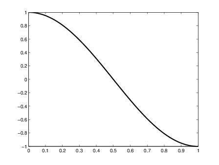
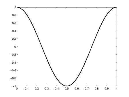
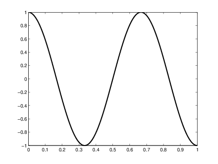
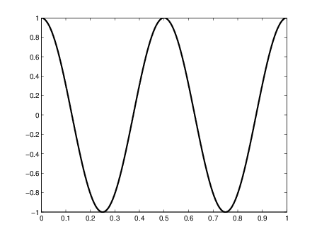
The Fourier Basis

The Fourier basis is a simple, principled basis function scheme for linear value function approximation in reinforcement learning. It has performed well over a wide range of problems, despite its simplicity, and I now use it almost exclusively. My advice to fellow researchers who require function approximation is that the Fourier basis should be the first thing you try.

If a problem is small enough, the Fourier basis avoids the need for extensive problem-specific feature engineering. For example, we have achieved good results on the Acrobot problem using a Fourier basis of order between 5 and 9; contrast this with the two paragraphs describing a problem-specific tile-coding originally used to solve the Acrobot. For larger problems, the Fourier basis provides a generic but complete basis function scheme suitable for feature selection.

For a single continuous state variable, $s$, (scaled to $[0,\; 1]$), the $n$th order Fourier basis is the set of basis functions defined as:

for $j\; \in \; [0,\; 1,\; ...,\; n]$. Thus, an order $n$ Fourier basis produces $n\; +\; 1$ basis functions, the first having value 1 everywhere. The following pictures show a few example basis functions; note that, as $j$ increases, the basis functions become higher frequency.

Univariate Fourier basis functions for $j\; =\; 1,\; 2,\; 3$ and $4$. The basis function for $j\; =\; 0$ is a constant.

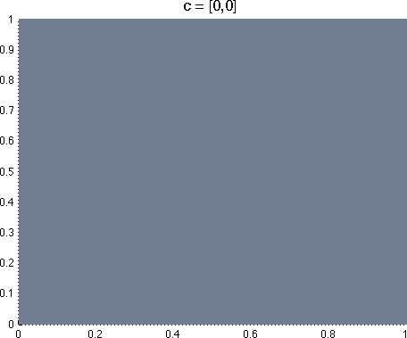
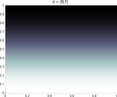
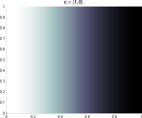
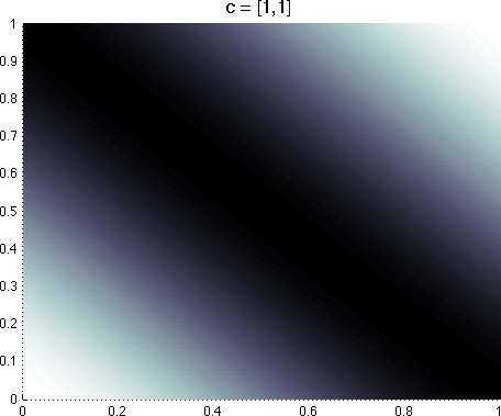
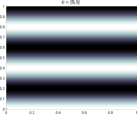
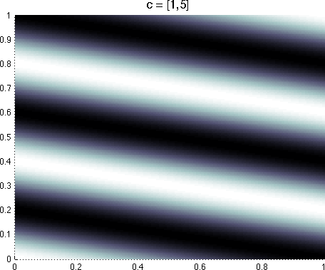
For multivariate state spaces, where $$s ∈ ℜ^d$(where\; each\; element$ s$$_i of $$s is scaled to $[0,\; 1]$) the $n$th order Fourier basis is defined by the set of basis functions:

where each c_j is a length $d$coefficient vector, each element of which is an integer between $0$ and $n$. The basis is obtained by enumerating all such coefficient vectors.

A few example basis functions for a 2D domain are shown below. Each element of the $$c_j vector specifies the basis function's frequency along the corresponding state variable; for example, in a 2D domain, $$c_j = [1, 2] results in a basis function with frequency $1$ along $s$₁ and frequency $2$ along $s$₂. Setting a state variable's coefficient to zero results in a basis function that is invariant to changes along that state dimension.

A few example Fourier basis functions defined over two state variables. Lighter colors indicate a value closer to $1$, darker colors indicate a value closer to $-1$.

One caveat: when performing gradient-descent style value function approximation (such as TD($\lambda$)), we must deal with the fact that some Fourier basis functions have much higher frequencies than others, and scale their gradient descent step sizes appropriately. In practice, we've found that setting $\alpha$_i = α₀/||c_i||₂, where $\alpha$₀ is the base learning rate assigned to the basis function with $$c₀, performs reliably well.

An $n$th order Fourier basis in a $d$-dimensional space has $(n\; +\; 1)d$ basis functions, and thus suffers the combinatorial explosion in $d$ exhibited by all complete fixed basis methods. In a domain where $d$ is sufficiently small - perhaps less than 6 or 7 - we may simply pick an order $n$ and enumerate all basis functions. This amounts to an expectation that components of the value function with frequency $n$ or less are signal, and components with higher frequency are noise. For higher dimensional domains, we may reduce the size of the basis by placing restrictions on the $$c_j vectors. For example, we can include only coefficient vectors with two or fewer non-zero elements; this is analogous to tile coding pairs of variables.

The paper describing the Fourier Basis is:

• G.D. Konidaris, S. Osentoski and P.S. Thomas. Value Function Approximation in Reinforcement Learning using the Fourier Basis. In Proceedings of the Twenty-Fifth Conference on Artificial Intelligence, pages 380-385, August 2011.

Source Code:

• An RL-Glue-compatible epsilon-greedy Sarsa(λ) agent is available on the RL Library community wiki. The code is in Java and is fully documented. (Apache License)


• A Python implementation of the Fourier basis, along with code for ε-greedy Sarsa(λ) and two RLGym examples, is available at: github.com/brownirl/fourier_vfa. (GPLv3 license)

Here is a list of papers using the Fourier basis, courtesy of Google Scholar.